04. Quiz: Log Returns and Compounding
Log Returns and Compounding
Log returns can be convenient for calculations that involve compounding. To explain this idea, let's first discuss compounding.
Annual Rate of Interest
SOLUTION:
$104Compounding
The idea of compounding is a simple one. Say you put $100 in a bank account that earns 4% interest per year, compounded annually. After 1 year, you have
$100 + $100*0.04 = $104.
The next year, you have,
$104 + $104*0.04 = $108.16,
so you earned another $4 of interest on the original $100 but also 16 cents on the $4 of interest earned last year.
Compounding is the process by which an asset’s earnings are reinvested to generate additional earnings, that is to say, earning interest on interest.
Rates of Compounding
SOLUTION:
$104.04Rates of Compounding
A statement by a bank that the interest rate on one-year deposits is 4% per year sounds straightforward and unambiguous. In fact, its precise meaning depends on the way the interest rate is measured. For an interest rate statement to be clear, the magnitude and time dependence of the rate of interest, as well as the frequency of compounding, must be clearly stated.
If the interest rate is measured with annual compounding, the bank’s statement that the interest rate is 4% means that $100 grows to \$100\times(1 + .04) = \$104 at the end of 1 year.
When the interest rate is measured with semiannual compounding, it means that 2% is earned every 6 months, with the interest being reinvested. In this case, $100 grows to \$100\times(1 + .04/2)\times(1 + .04/2) = \$100\times(1 + .04/2)^2 = \$104.04 , at the end of 1 year.
When the interest rate is measured with quarterly compounding, the bank’s statement means that 1% is earned every 3 months, with the interest being reinvested. The $100 then grows to \$100\times(1 + .04/4)^4 = \$104.06 at the end of 1 year.
Continuous Compounding
Let's compare the amount of money accumulated after 1 year with the same annual rate of interest of 4%, but different rates of compounding:
\begin{array}{c c} \textbf{Compounding frequency} & \textbf{Value of \$100 after 1 year} \\ \textrm{Annually (n=1)} & \$104.00 \\ \textrm{Semi-annually (n=2)} & \$104.04 \\ \textrm{Quarterly (n=4)} & \$104.06 \\ \textrm{Monthly (n=12)} & \$104.07 \\ \textrm{Weekly (n=52)} & \$104.08 \\ \textrm{Daily (n=252)} & \$104.08\end{array}
Looking at the table, you can see that with more frequent compounding, the value at 1 year increases but then seems to level off. If you assumed that the benefit of compounding more and more frequently had a limit, you would be right! How do we calculate this limit? Well, first we write down the formula for compounding,
p_t = p_{t-1}(1 + \frac{r}{n})^n ,
and then we notice that what we'd like to do is make n bigger and bigger. We want the limit as n goes to infinity. Well, it turns out that this limit is:
\lim_{n\to\infty}\left( 1 + \frac{r}{n}\right)^n = \mathrm{e}^r
Compounding infinitely often is called continuous compounding . So what does this mean? Well, it means that if you wanted to calculate how much money you’d have at the end of the year if you started with $100 and compounded continuously , but at a simple annual rate of 4%, you’d calculate:
\$100 \times \mathrm{e}^{.04} = \$104.08
You'll notice that the value after 1 year with continuous compounding is pretty close (it's the same if we round to two decimal places) to the value after 1 year with daily compounding.
Continuously Compounded Return
Now, say you were trying to reverse the previous calculation. Say you knew you had $104.08 at the end of the year, and $100 at the beginning of the year, and you wanted to calculate the rate of interest as if it had been compounded continuously . You would simply invert the formula. So you’d calculate:
\$104.08/\$100 = \mathrm{e}^r
Then you'd take the natural log of both sides, and then you'd have,
\ln(\$104.08/\$100) = r
So,
.04 = r
r is the continuously compounded annual return . So the continuously compounded annual return equals \ln(p_t/p_{t-1}) . But what is this quantity? It’s just the log return! This is why you might hear log returns called continuously compounded returns .
Additivity
Now, say we invested $100, and the monthly continuously compounded interest rate was 2%. At the end of the month, we’d have
\$100 \times \mathrm{e}^{.02} = \$102.02
But if the investment continued to accrue at a monthly continuously compounded rate of 0.02 for a whole year, we’d have
\$100 \times \mathrm{e}^{.02}\times \mathrm{e}^{.02}\times \mathrm{e}^{.02}\times \mathrm{e}^{.02}\times \mathrm{e}^{.02}\times \mathrm{e}^{.02}\times \mathrm{e}^{.02}\times \mathrm{e}^{.02}\times \mathrm{e}^{.02}\times \mathrm{e}^{.02}\times \mathrm{e}^{.02}\times \mathrm{e}^{.02}
… in total, 12 factors of
\mathrm{e}^{.02}
.
So we'd have
\$100 \times (\mathrm{e}^{.02*12}) = \$127.12
Equivalently,
\$100 \times \mathrm{e}^{.24} = \$127.12
Since the annual rate of continuous compounding, 0.24, is simply the sum of the monthly rates of continuous compounding, we say that the continuously compounded rate of return is additive over time .
Annualized Rate of Return
We saw above how to calculate the annual rate of continuous compounding from the monthly rate of continuous compounding. If we just had a single monthly rate, but we assumed that the rates for all the months of the year were the same, we could extrapolate the monthly rate to an annual rate by multiplying by 12. This is called annualizing the rate of continuous compounding. Rates of return and other metrics are often converted to a common annual basis in order to make comparisons across contexts and instruments.
Time Additivity of Log Returns
So, as you can see, the rate of continuous compounding is additive over time. Since, mathematically, the rate of continuous compounding is just the log return, this means that log returns are additive over time, and this can be very convenient. As another example,
\mathrm{log\;return\;for\;January} + \mathrm{log\;return\;for\;February}
= \ln \left( \frac{p_{\mathrm{Feb\;1}}}{p_{\mathrm{Jan\;1}}} \right) + \ln \left( \frac{p_{\mathrm{Mar\;1}}}{p_{\mathrm{Feb\;1}}} \right)
= \ln(p_{\mathrm{Feb\;1}}) - \ln(p_{\mathrm{Jan\;1}}) + \ln(p_{\mathrm{Mar\;1}}) - \ln(p_{\mathrm{Feb\;1}})
= \ln(p_{\mathrm{Mar\;1}}) - \ln(p_{\mathrm{Jan\;1}})
= \ln \left( \frac{p_{\mathrm{Mar\;1}}}{p_{\mathrm{Jan\;1}}} \right)
=\mathrm{log\;return\;for\;January\;and\;February}
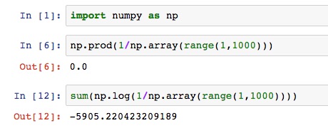
Numerical Stability
Multiplication of many small numbers can result in the problem that the product is smaller than the smallest number representable in computer memory. Sometimes the computation will incorrectly yield the value 0. This is called arithmetic underflow . The use of logarithms can help with this, since it enables the representation of much smaller (and much larger) numbers. For example: